Μετάβαση στο κύριο περιεχόμενο

Πώς να μορφοποιήσετε υπό όρους βάσει ενός άλλου φύλλου στο φύλλο Google;

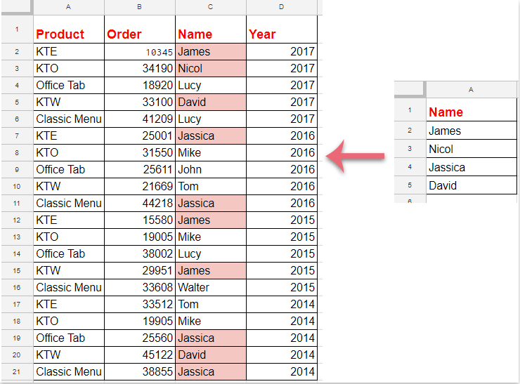
Εάν θέλετε να εφαρμόσετε τη μορφοποίηση υπό όρους για να επισημάνετε κελιά με βάση μια λίστα δεδομένων από άλλο φύλλο, όπως το παρακάτω στιγμιότυπο οθόνης που εμφανίζεται στο φύλλο Google, έχετε εύκολες και καλές μεθόδους για την επίλυσή του;

Μορφοποίηση υπό όρους για την επισήμανση κελιών με βάση μια λίστα από άλλο φύλλο στα Φύλλα Google


Μορφοποίηση υπό όρους για την επισήμανση κελιών με βάση μια λίστα από άλλο φύλλο στα Φύλλα Google


Κάντε τα ακόλουθα βήματα για να ολοκληρώσετε αυτήν την εργασία:

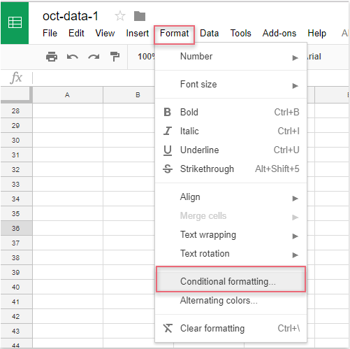
1. Κλίκ Μορφή > Μορφοποίηση υπό όρους, δείτε το στιγμιότυπο οθόνης:

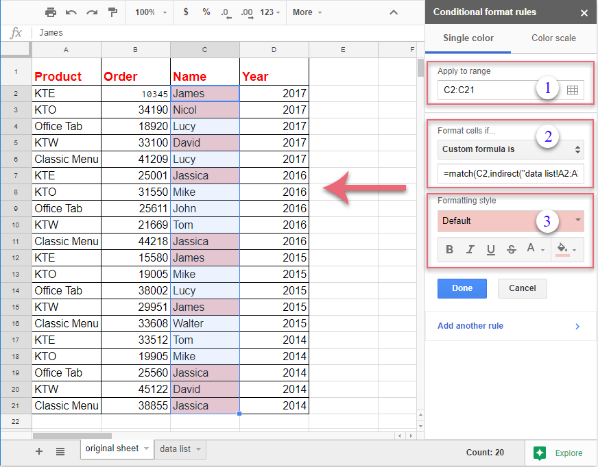
2. Στην Κανόνες μορφής υπό όρους παράθυρο, κάντε τις ακόλουθες λειτουργίες:

(1.) Κάντε κλικ κουμπί για να επιλέξετε τα δεδομένα στηλών που θέλετε να επισημάνετε.

(2.) Στο Μορφοποίηση κελιών εάν αναπτυσσόμενη λίστα, επιλέξτε Ο συνήθης τύπος είναι και, στη συνέχεια, εισαγάγετε αυτόν τον τύπο: =match(C2,έμμεσο("λίστα δεδομένων!A2:A"),0) στο πλαίσιο κειμένου.

(3.) Στη συνέχεια, επιλέξτε μία μορφοποίηση από το Στυλ μορφοποίησης όπως χρειάζεστε.

Note: Στον παραπάνω τύπο: C2 είναι το πρώτο κελί των δεδομένων της στήλης που θέλετε να επισημάνετε και το λίστα δεδομένων! A2: A είναι το όνομα φύλλου και το εύρος κελιών λίστας που περιέχει τα κριτήρια στα οποία θέλετε να επισημάνετε τα κελιά με βάση.

3. Και όλα τα κελιά που ταιριάζουν με βάση τα κελιά της λίστας έχουν επισημανθεί ταυτόχρονα και, στη συνέχεια, πρέπει να κάνετε κλικ στο Ολοκληρώθηκε για να κλείσετε το Κανόνες μορφής υπό όρους τζάμι όπως χρειάζεστε.


Τα καλύτερα εργαλεία παραγωγικότητας γραφείου

🤖 Kutools AI Aide: Επανάσταση στην ανάλυση δεδομένων με βάση: Ευφυής Εκτέλεση   |  Δημιουργία κώδικα  |  Δημιουργία προσαρμοσμένων τύπων  |  Αναλύστε δεδομένα και δημιουργήστε γραφήματα  |  Επίκληση Λειτουργιών Kutools...
Δημοφιλή χαρακτηριστικά: Εύρεση, επισήμανση ή αναγνώριση διπλότυπων   |  Διαγραφή κενών γραμμών   |  Συνδυάστε στήλες ή κελιά χωρίς απώλεια δεδομένων   |   Γύρος χωρίς φόρμουλα ...
Σούπερ Αναζήτηση: VLookup πολλαπλών κριτηρίων    VLookup πολλαπλών τιμών  |   VLookup σε πολλά φύλλα   |   Ασαφής αναζήτηση ....
Σύνθετη αναπτυσσόμενη λίστα: Γρήγορη δημιουργία αναπτυσσόμενης λίστας   |  Εξαρτημένη αναπτυσσόμενη λίστα   |  Πολλαπλή αναπτυσσόμενη λίστα ....
Διαχειριστής στήλης: Προσθέστε έναν συγκεκριμένο αριθμό στηλών  |  Μετακίνηση στηλών  |  Εναλλαγή κατάστασης ορατότητας κρυφών στηλών  |  Συγκρίνετε εύρη και στήλες ...
Επιλεγμένα Χαρακτηριστικά: Εστίαση πλέγματος   |  Προβολή σχεδίου   |   Μεγάλη Formula Bar    Διαχείριση βιβλίου εργασίας & φύλλου   |  Βιβλιοθήκη πόρων (Αυτόματο κείμενο)   |  Επιλογή ημερομηνίας   |  Συνδυάστε φύλλα εργασίας   |  Κρυπτογράφηση/Αποκρυπτογράφηση κελιών    Αποστολή email ανά λίστα   |  Σούπερ φίλτρο   |   Ειδικό φίλτρο (φίλτρο με έντονη γραφή/πλάγια γραφή/διαγραφή...) ...
Κορυφαία 15 σύνολα εργαλείων12 Κείμενο Εργαλεία (Προσθήκη κειμένου, Κατάργηση χαρακτήρων, ...)   |   50 + Διάγραμμα Τύποι (Gantt διάγραμμα, ...)   |   40+ Πρακτικό ΜΑΘΗΜΑΤΙΚΟΙ τυποι (Υπολογίστε την ηλικία με βάση τα γενέθλια, ...)   |   19 Εισαγωγή Εργαλεία (Εισαγωγή κωδικού QR, Εισαγωγή εικόνας από το μονοπάτι, ...)   |   12 Μετατροπή Εργαλεία (Αριθμοί σε λέξεις, Μετατροπή Συναλλάγματος, ...)   |   7 Συγχώνευση & διαχωρισμός Εργαλεία (Σύνθετες σειρές συνδυασμού, Διαίρεση κελιών, ...)   |   ... κι αλλα

Αυξήστε τις δεξιότητές σας στο Excel με τα Kutools για Excel και απολαύστε την αποτελεσματικότητα όπως ποτέ πριν. Το Kutools για Excel προσφέρει πάνω από 300 προηγμένες δυνατότητες για την ενίσχυση της παραγωγικότητας και την εξοικονόμηση χρόνου.  Κάντε κλικ εδώ για να αποκτήσετε τη δυνατότητα που χρειάζεστε περισσότερο...

Περιγραφή


Το Office Tab φέρνει τη διεπαφή με καρτέλες στο Office και κάνει την εργασία σας πολύ πιο εύκολη

  • Ενεργοποίηση επεξεργασίας και ανάγνωσης καρτελών σε Word, Excel, PowerPoint, Publisher, Access, Visio και Project.
  • Ανοίξτε και δημιουργήστε πολλά έγγραφα σε νέες καρτέλες του ίδιου παραθύρου και όχι σε νέα παράθυρα.
  • Αυξάνει την παραγωγικότητά σας κατά 50% και μειώνει εκατοντάδες κλικ του ποντικιού για εσάς κάθε μέρα!


Comments (27)
Rated 5 out of 5 · 2 ratings
This comment was minimized by the moderator on the site
Hi! skyyang ! Thank you, =match(C2,indirect("data list!A2:A"),0) works for me.

But I would like to format more than one column, so column A in sheet a is checked against column B in sheet b , and so.
There are so many columns so I can not apply one format per column, but a whole conditional format for the whole sheet.


How should I modify the range and the formula?

Thanks!
This comment was minimized by the moderator on the site
What if the cell values you're trying to match are hyperlinks?
Rated 5 out of 5
This comment was minimized by the moderator on the site
Pardon, il fallait lire =A1<>INDIRECT("PreviousVersion!"& CHAR (COLUMN () + 64) & ROW ()) ...
This comment was minimized by the moderator on the site
Bonjour,
J'ai une autre question du même type au sujet d'un formatage conditionnel qui fonctionne sur Excel mais que je n'arrive pas à porter sur Google Sheet :
L'idée est de comparer 2 versions d'une même feuille que l'on stock à l'aide de 2 onglets (2 feuilles du même workbook)

La formule est la suivante : =A1<>'previousVersion'!A1 avec un formatage fond jaune pour mettre en évidence les changements sur toute la feuille car l'idée est d'appliquer ce
formatage conditionnel sur toutes les cellules de la feuille ($A$1:$V:1000)

Sur Google sheet cette formule m'est interdite et si je passe par un "indirect("previousVersion!A1"), je perds le coté dynamique sur le "A1" de la feuille precious version
Si j'essaye =A1<>indirect("previousVersion!"&A1) j'ai une erreur car c'est la valeur de A1 qui est interprétée et concaténée avec "previousVersion!"

Si j'essaye la formule =C3<>INDIRECT("PreviousVersion!"& CHAR (COLUMN () + 64) & ROW ()) cela ne fonctionne pas non plus....

Si vous avez une solution...
Merci d'avance
This comment was minimized by the moderator on the site
Bonjour,
Dans Feuille google je cherche la formule suivante
Si dans la cel A1 = text alors dans la Cel B1 ecire telle valeur ou texte automatiquement
Merci d avance pour votre aide
This comment was minimized by the moderator on the site
What if it's not an exact match but contains the reference data.
This comment was minimized by the moderator on the site
Hello, ashley
To solve your problem, please apply the below formula:
=REGEXMATCH(C2:C21,INDIRECT("Sheet2!$A$2"))

Please try, hope it can help you!
This comment was minimized by the moderator on the site
What happens if the data in my list is in more than one column? When I try to use datalist!A2:M or datalist!A:M or datalist!A2:M17 none of those work.
This comment was minimized by the moderator on the site
I have even tried naming the specific range I want to refer to and using that in the formula, no luck.
This comment was minimized by the moderator on the site
How to highlight the entire row data with conditional formatting using other sub-sheet
This comment was minimized by the moderator on the site
Hello, Ranganath
To highlight the entire row based on the data list, please do as this:
1. In the Apply to range box, select the whole sheet;
2. Apply this formula: =match($C2,indirect("datalist!A2:A"),0) into the Custom formula is textbox.
Please try, hope it can help you!

https://www.extendoffice.com/images/stories/comments/comment-skyyang/doc-highlight-entire-row.png
This comment was minimized by the moderator on the site
Hey, Thanks for replying. I have tried the formula but its not working.
Rated 5 out of 5
This comment was minimized by the moderator on the site
Hi,
Have you modified the sheet name and cell reference to your own data?
$C2 is the first cell of the column data that you want to highlight, and the datalist!A2:A is another sheet name and list range which contains the criteria you want to highlight the cells based on.
Please check them, thank you!
This comment was minimized by the moderator on the site
This doesn't work for me. I have triple checked everything.

Apply to range: K1:K2158

=match(K2,indirect("TorontoCitys!A1:A"),0)

It highlights random other city names, not in the TorontoCity's list.

K2 (is my main sheet and the starting column cell of the column I want to be affected.
TorontoCitys (is the name of the sheet)
A1 is the start of the column of the list of city names.
A is the column.

Could be that my punctuation's are incorrect?

Thanks in advance.
This comment was minimized by the moderator on the site
Hello friend,

Glad to help. Your formula is correct, please don't worry. The problem is the range you apply to. It shouldn't be K1:K2158, but K2:K2158.

Please see the screenshots. The example is simple but enough to explain the problem.

The correct "Apply to Range" is A2:A20. And the correct formula is =match(A2,indirect("TorontoCitys!A1:A"),0). Then correct cities can be highlighted. Please see screenshot 2.
But if I change the "Apply to Range" to A1:A20, the wrong city name is highlighted. Please see screenshot 3.

So please change your "Apply to Range" from K1:K2158 to K2:K2158. The problem should be solved. Looking forward to your reply.

Sincerely,
Mandy
This comment was minimized by the moderator on the site
how do you do this but with the entire row highlighted
There are no comments posted here yet
Load More
Please leave your comments in English
Posting as Guest
×
Rate this post:
0   Characters
Suggested Locations