Μετάβαση στο κύριο περιεχόμενο

Πώς να αναζητήσετε την πρώτη μη μηδενική τιμή και να επιστρέψετε την αντίστοιχη κεφαλίδα στήλης στο Excel;

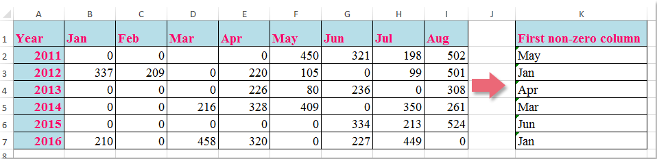
Υποθέτοντας ότι έχετε μια σειρά δεδομένων, τώρα, θέλετε να επιστρέψετε την κεφαλίδα στήλης σε αυτήν τη σειρά όπου εμφανίζεται η πρώτη μη μηδενική τιμή όπως φαίνεται στο παρακάτω στιγμιότυπο οθόνης, αυτό το άρθρο, θα εισαγάγω έναν χρήσιμο τύπο για να αντιμετωπίσετε αυτήν την εργασία στο Excel.

αναζήτηση εγγράφου πρώτη μη μηδενική 1

Αναζητήστε την πρώτη μη μηδενική τιμή και επιστρέψτε την αντίστοιχη κεφαλίδα στήλης με τύπο


βέλος μπλε δεξιά φούσκα Αναζητήστε την πρώτη μη μηδενική τιμή και επιστρέψτε την αντίστοιχη κεφαλίδα στήλης με τύπο

Για να επιστρέψετε την κεφαλίδα στήλης της πρώτης μη μηδενικής τιμής στη σειρά, ο ακόλουθος τύπος μπορεί να σας βοηθήσει, κάντε ως εξής:

Εισαγάγετε αυτόν τον τύπο: =INDEX($B$1:$I$1,MATCH(TRUE,INDEX(B2:I2<>0,),0)) σε ένα κενό κελί όπου θέλετε να εντοπίσετε το αποτέλεσμα, K2, για παράδειγμα, και, στη συνέχεια, σύρετε τη λαβή πλήρωσης προς τα κάτω στα κελιά που θέλετε να εφαρμόσετε αυτόν τον τύπο και όλες οι αντίστοιχες κεφαλίδες στηλών της πρώτης μη μηδενικής τιμής επιστρέφονται ως το ακόλουθο στιγμιότυπο οθόνης:

αναζήτηση εγγράφου πρώτη μη μηδενική 2

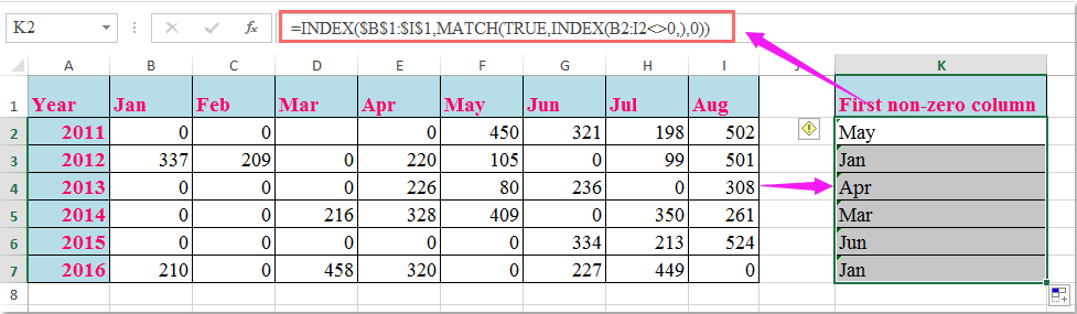
Note: Στον παραπάνω τύπο, Β1: I1 είναι οι κεφαλίδες στηλών που θέλετε να επιστρέψετε, Β2: I2 είναι τα δεδομένα σειράς που θέλετε να αναζητήσετε την πρώτη μη μηδενική τιμή.

Τα καλύτερα εργαλεία παραγωγικότητας γραφείου

🤖 Kutools AI Aide: Επανάσταση στην ανάλυση δεδομένων με βάση: Ευφυής Εκτέλεση   |  Δημιουργία κώδικα  |  Δημιουργία προσαρμοσμένων τύπων  |  Αναλύστε δεδομένα και δημιουργήστε γραφήματα  |  Επίκληση Λειτουργιών Kutools...
Δημοφιλή χαρακτηριστικά: Εύρεση, επισήμανση ή αναγνώριση διπλότυπων   |  Διαγραφή κενών γραμμών   |  Συνδυάστε στήλες ή κελιά χωρίς απώλεια δεδομένων   |   Γύρος χωρίς φόρμουλα ...
Σούπερ Αναζήτηση: VLookup πολλαπλών κριτηρίων    VLookup πολλαπλών τιμών  |   VLookup σε πολλά φύλλα   |   Ασαφής αναζήτηση ....
Σύνθετη αναπτυσσόμενη λίστα: Γρήγορη δημιουργία αναπτυσσόμενης λίστας   |  Εξαρτημένη αναπτυσσόμενη λίστα   |  Πολλαπλή αναπτυσσόμενη λίστα ....
Διαχειριστής στήλης: Προσθέστε έναν συγκεκριμένο αριθμό στηλών  |  Μετακίνηση στηλών  |  Εναλλαγή κατάστασης ορατότητας κρυφών στηλών  |  Συγκρίνετε εύρη και στήλες ...
Επιλεγμένα Χαρακτηριστικά: Εστίαση πλέγματος   |  Προβολή σχεδίου   |   Μεγάλη Formula Bar    Διαχείριση βιβλίου εργασίας & φύλλου   |  Βιβλιοθήκη πόρων (Αυτόματο κείμενο)   |  Επιλογή ημερομηνίας   |  Συνδυάστε φύλλα εργασίας   |  Κρυπτογράφηση/Αποκρυπτογράφηση κελιών    Αποστολή email ανά λίστα   |  Σούπερ φίλτρο   |   Ειδικό φίλτρο (φίλτρο με έντονη γραφή/πλάγια γραφή/διαγραφή...) ...
Κορυφαία 15 σύνολα εργαλείων12 Κείμενο Εργαλεία (Προσθήκη κειμένου, Κατάργηση χαρακτήρων, ...)   |   50 + Διάγραμμα Τύποι (Gantt διάγραμμα, ...)   |   40+ Πρακτικό ΜΑΘΗΜΑΤΙΚΟΙ τυποι (Υπολογίστε την ηλικία με βάση τα γενέθλια, ...)   |   19 Εισαγωγή Εργαλεία (Εισαγωγή κωδικού QR, Εισαγωγή εικόνας από το μονοπάτι, ...)   |   12 Μετατροπή Εργαλεία (Αριθμοί σε λέξεις, Μετατροπή Συναλλάγματος, ...)   |   7 Συγχώνευση & διαχωρισμός Εργαλεία (Σύνθετες σειρές συνδυασμού, Διαίρεση κελιών, ...)   |   ... κι αλλα

Αυξήστε τις δεξιότητές σας στο Excel με τα Kutools για Excel και απολαύστε την αποτελεσματικότητα όπως ποτέ πριν. Το Kutools για Excel προσφέρει πάνω από 300 προηγμένες δυνατότητες για την ενίσχυση της παραγωγικότητας και την εξοικονόμηση χρόνου.  Κάντε κλικ εδώ για να αποκτήσετε τη δυνατότητα που χρειάζεστε περισσότερο...

Περιγραφή


Το Office Tab φέρνει τη διεπαφή με καρτέλες στο Office και κάνει την εργασία σας πολύ πιο εύκολη

  • Ενεργοποίηση επεξεργασίας και ανάγνωσης καρτελών σε Word, Excel, PowerPoint, Publisher, Access, Visio και Project.
  • Ανοίξτε και δημιουργήστε πολλά έγγραφα σε νέες καρτέλες του ίδιου παραθύρου και όχι σε νέα παράθυρα.
  • Αυξάνει την παραγωγικότητά σας κατά 50% και μειώνει εκατοντάδες κλικ του ποντικιού για εσάς κάθε μέρα!
Comments (15)
No ratings yet. Be the first to rate!
This comment was minimized by the moderator on the site
Hello, my problem is: a have value 1,2,3,4,...50 that are the number of month. How to denormalize month into real datum. Thank you in advance a lot!!!
This comment was minimized by the moderator on the site
Does anyone know what you would do if your cell that contains a zero has a formula in it? When I use this formula, I end up with whatever the first column header is regardless of whether it is zero or not.
This comment was minimized by the moderator on the site
E como faço pra procurar o primeiro valor diferente de zero da esquerda pra direita?
This comment was minimized by the moderator on the site
Hello, Matheus
If you want to return the first non-zero value from a row, please apply the below formula:
=INDEX(B2:F2,MATCH(TRUE,INDEX(B2:F2<>0,),0))
Please have a try, hope it can help you!
This comment was minimized by the moderator on the site
What if you needed the last non-zero value in an array?

P.S. This was really helpful, thank you so much!
This comment was minimized by the moderator on the site
Hello, Ali,
To get the column header based on the last non-zero value, please apply the below formula, see screenshot:
=INDEX($B$1:$H$1,MAX((COLUMN(B2:H2)-MIN(COLUMN(B2:H2))+1)*(B2:H2<>0)))
Please remember to press Ctrl+Shift+Enter key together.
https://www.extendoffice.com/images/stories/comments/comment-skyyang/doc-last-non-zero.png
Please try, hope it can help you!
This comment was minimized by the moderator on the site
The formula is super helpful and helped me sorted out the situation! Thanks!!! Is there any chance you may please help to also explain how it works?
This comment was minimized by the moderator on the site
How do you look up for the second,third and fourth non-zero value?
This comment was minimized by the moderator on the site
Hello, Robert,
To lookup the second, third or fourth non-zero values and return their columns, please apply the below formula: (After pasting the formula, please press Ctr + Shift + Enter keys together.)
=INDEX($B$1:$I$1,SMALL(IF(B2:I2<>0, COLUMN(B2:I2)-COLUMN(A2)),2))


Note: To extract the third or fourth result, you just need to change the number 2 to 3,4 as you need.

Please have a try, hope it can help you!
This comment was minimized by the moderator on the site
CAN U EXPLIAN HOW THIS FORMULA WORKS
This comment was minimized by the moderator on the site
Hello Priya,I am glad to help. I will separate the formula = INDEX($B$1:$I$1,MATCH(TRUE,INDEX(B2:I2<>0,),0)) into 3 parts, and explain the formula to you step by step.
First, let us see the inner-most formula =INDEX(B2:I2<>0,). This formula returns an array of TRUE and FALSE whether the values of range B2:I2 are equal to 0. Please see the screenshot 1, formula =INDEX(B2:I2<>0,) returns {FALSE,FALSE,FALSE,FALSE,TRUE,TRUE,TRUE,TRUE}.
Second, =MATCH(TRUE,INDEX(B2:I2<>0,),0) =MATCH(TRUE, {FALSE,FALSE,FALSE,FALSE,TRUE,TRUE,TRUE,TRUE}, 0). It returns the position of the first value "TRUE", while 0 in the formula means an exact match. We can see that the first value "TRUE" occurs at the 5th position of the array. Then the second formula returns 5. See the screenshot 2.
Finally,  =INDEX(B1:I1,MATCH(TRUE,INDEX(B2:I2<>0,),0))=INDEX(B1:I1,5). It returns the 5th value of the array B1:I1. We can see in the screenshot that the value is "May". So the final formula returns "May". 
PS: To drag the fill handle down the formula to get the rest of the results, we must make the range B1:I1 absolute. So we add $ to range B1:I1 to keep it absolute. 
Hope my explanation can solve your puzzle. Have a nice day.
Sincerely,Mandy
This comment was minimized by the moderator on the site
Thank you Mandy for illustrating it in detail.
Kindly guide how to get the last non zero value from same formula instead of first non zero value.
Will Match work for that or not?
This comment was minimized by the moderator on the site
Hi MandyZhou,

Thank you for the explanation!
I have a follow-up question.
How would the formula change if you had to look up the year too?
So in the above example, let's assume that column J is 'Year' and that in cell J2 is written '2015'.
And in cell K2 I would need the column header for the first non-zero value of the year in L2 (year 2015, so I would need to find 'Jun' in cell K2).

Thanks in advance for your help!
Jason
This comment was minimized by the moderator on the site
How can I return the second and third, etc non zero value? Your formula is amazing but I am trying to search more keywords from a text so sometimes they are 2 or 3 in the same sentence
This comment was minimized by the moderator on the site
se volessi "l'ultimo" Valore Diverso Da Zero E Restituire L'intestazione Della Colonna Corrispondente Con La Formula?
There are no comments posted here yet
Please leave your comments in English
Posting as Guest
×
Rate this post:
0   Characters
Suggested Locations