Μετάβαση στο κύριο περιεχόμενο

Πώς να επιστρέψετε πολλές τιμές αντιστοίχισης με βάση ένα ή περισσότερα κριτήρια στο Excel;

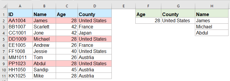
Κανονικά, αναζητήστε μια συγκεκριμένη τιμή και επιστρέψτε το αντίστοιχο στοιχείο είναι εύκολο για τους περισσότερους από εμάς χρησιμοποιώντας τη λειτουργία VLOOKUP. Ωστόσο, έχετε προσπαθήσει ποτέ να επιστρέψετε πολλές τιμές αντιστοίχισης με βάση ένα ή περισσότερα κριτήρια, όπως φαίνεται στο παρακάτω στιγμιότυπο οθόνης; Σε αυτό το άρθρο, θα παρουσιάσω ορισμένους τύπους για την επίλυση αυτής της σύνθετης εργασίας στο Excel.

Επιστρέψτε πολλές τιμές αντιστοίχισης με βάση ένα ή περισσότερα κριτήρια με τύπους πίνακα


Επιστρέψτε πολλές τιμές αντιστοίχισης με βάση ένα ή περισσότερα κριτήρια με τύπους πίνακα

Για παράδειγμα, θέλω να εξαγάγω όλα τα ονόματα των οποίων η ηλικία είναι 28 ετών και προέρχονται από Ηνωμένες Πολιτείες, εφαρμόστε τον ακόλουθο τύπο:

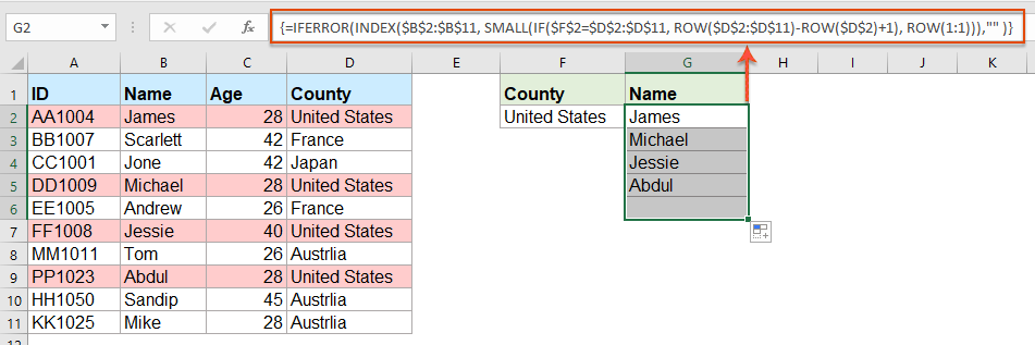
1. Αντιγράψτε ή εισαγάγετε τον παρακάτω τύπο σε ένα κενό κελί όπου θέλετε να εντοπίσετε το αποτέλεσμα:

=INDEX($B$2:$B$11, SMALL(IF(COUNTIF($F$2, $C$2:$C$11)*COUNTIF($G$2, $D$2:$D$11), ROW($A$2:$D$11)-MIN(ROW($A$2:$D$11))+1), ROW(A1)), COLUMN(A1))

Note: Στον παραπάνω τύπο, Β2: Β11 είναι η στήλη από την οποία επιστρέφεται η αντίστοιχη τιμή. F2, C2: C11 είναι η πρώτη συνθήκη και τα δεδομένα της στήλης που περιέχουν την πρώτη συνθήκη. G2, D2: D11 είναι η δεύτερη συνθήκη και τα δεδομένα της στήλης που περιέχουν αυτήν την κατάσταση, αλλάξτε τα ανάλογα με τις ανάγκες σας.

2. Στη συνέχεια, πατήστε Ctrl + Shift + Εισαγωγή για να λάβετε το πρώτο αποτέλεσμα αντιστοίχισης και, στη συνέχεια, επιλέξτε το πρώτο κελί τύπου και σύρετε τη λαβή πλήρωσης προς τα κάτω έως ότου εμφανιστεί η τιμή σφάλματος, τώρα, όλες οι τιμές αντιστοίχισης επιστρέφονται όπως φαίνεται στο παρακάτω στιγμιότυπο οθόνης:

Συμβουλές: Εάν απλώς πρέπει να επιστρέψετε όλες τις αντίστοιχες τιμές με βάση μία συνθήκη, εφαρμόστε τον παρακάτω τύπο πίνακα:

=IFERROR(INDEX($B$2:$B$11, SMALL(IF($F$2=$D$2:$D$11, ROW($D$2:$D$11)-ROW($D$2)+1), ROW(1:1))),"" )


Σχετικά άρθρα:

  • Επιστροφή πολλαπλών τιμών αναζήτησης σε ένα κελί διαχωρισμένο με κόμμα
  • Στο Excel, μπορούμε να εφαρμόσουμε τη συνάρτηση VLOOKUP για να επιστρέψουμε την πρώτη αντιστοιχισμένη τιμή από κελιά πίνακα, αλλά, μερικές φορές, πρέπει να εξαγάγουμε όλες τις τιμές που ταιριάζουν και στη συνέχεια να διαχωρίζονται από ένα συγκεκριμένο οριοθέτη, όπως κόμμα, παύλα κ.λπ. ... σε ένα μόνο κελί όπως φαίνεται το ακόλουθο στιγμιότυπο οθόνης. Πώς θα μπορούσαμε να πάρουμε και να επιστρέψουμε πολλές τιμές αναζήτησης σε ένα κελί διαχωρισμένο με κόμμα στο Excel;
  • Vlookup και επιστροφή πολλαπλών τιμών αντιστοίχισης ταυτόχρονα στο φύλλο Google
  • Η κανονική συνάρτηση Vlookup στο φύλλο Google μπορεί να σας βοηθήσει να βρείτε και να επιστρέψετε την πρώτη τιμή αντιστοίχισης με βάση δεδομένα δεδομένα. Ωστόσο, μερικές φορές, ίσως χρειαστεί να δείτε και να επιστρέψετε όλες τις αντίστοιχες τιμές όπως φαίνεται στο παρακάτω στιγμιότυπο οθόνης. Έχετε καλούς και εύκολους τρόπους για να επιλύσετε αυτήν την εργασία στο φύλλο Google;
  • Vlookup και επιστροφή πολλαπλών τιμών από την αναπτυσσόμενη λίστα
  • Στο Excel, πώς θα μπορούσατε να προβάλετε και να επιστρέψετε πολλές αντίστοιχες τιμές από μια αναπτυσσόμενη λίστα, πράγμα που σημαίνει ότι όταν επιλέγετε ένα στοιχείο από την αναπτυσσόμενη λίστα, όλες οι σχετικές τιμές εμφανίζονται ταυτόχρονα όπως φαίνεται στο παρακάτω στιγμιότυπο οθόνης. Αυτό το άρθρο, θα παρουσιάσω τη λύση βήμα προς βήμα.
  • Vlookup και επιστροφή πολλαπλών τιμών κάθετα στο Excel
  • Κανονικά, μπορείτε να χρησιμοποιήσετε τη συνάρτηση Vlookup για να λάβετε την πρώτη αντίστοιχη τιμή, αλλά, μερικές φορές, θέλετε να επιστρέψετε όλες τις εγγραφές που ταιριάζουν με βάση ένα συγκεκριμένο κριτήριο. Αυτό το άρθρο, θα μιλήσω για το πώς να βλέπω και να επιστρέφω όλες τις αντίστοιχες τιμές κάθετα, οριζόντια ή σε ένα μόνο κελί.
  • Vlookup και Return Data Matching μεταξύ δύο τιμών στο Excel
  • Στο Excel, μπορούμε να εφαρμόσουμε τη συνήθη συνάρτηση Vlookup για να λάβουμε την αντίστοιχη τιμή βάσει ενός δεδομένου δεδομένων. Αλλά, μερικές φορές, θέλουμε να κοιτάξουμε και να επιστρέψουμε την αντίστοιχη τιμή μεταξύ δύο τιμών όπως φαίνεται στο παρακάτω στιγμιότυπο οθόνης, πώς θα μπορούσατε να αντιμετωπίσετε αυτήν την εργασία στο Excel;


  • Super Formula Bar (επεξεργαστείτε εύκολα πολλές γραμμές κειμένου και τύπου). Διάταξη ανάγνωσης (εύκολη ανάγνωση και επεξεργασία μεγάλου αριθμού κελιών). Επικόλληση σε φιλτραρισμένο εύρος...
  • Συγχώνευση κελιών / σειρών / στηλών και τήρηση δεδομένων · Περιεχόμενο διαχωρισμού κελιών Συνδυάστε διπλές σειρές και άθροισμα / μέσος όρος... Αποτροπή διπλών κυττάρων; Συγκρίνετε τα εύρη...
  • Επιλέξτε Διπλότυπο ή Μοναδικό Σειρές; Επιλέξτε Κενές σειρές (όλα τα κελιά είναι κενά). Σούπερ εύρεση και ασαφής εύρεση σε πολλά βιβλία εργασίας. Τυχαία επιλογή ...
  • Ακριβές αντίγραφο Πολλαπλά κελιά χωρίς αλλαγή της αναφοράς τύπου. Αυτόματη δημιουργία αναφορών σε πολλαπλά φύλλα? Εισαγωγή κουκκίδων, Πλαίσια ελέγχου και άλλα ...
  • Αγαπημένα και γρήγορη εισαγωγή τύπων, Σειρά, Διαγράμματα και Εικόνες; Κρυπτογράφηση κυττάρων με κωδικό πρόσβασης Δημιουργία λίστας αλληλογραφίας και στείλτε email ...
  • Εξαγωγή κειμένου, Προσθήκη κειμένου, Κατάργηση κατά θέση, Αφαιρέστε το διάστημα; Δημιουργία και εκτύπωση υποσύνολων σελιδοποίησης. Μετατροπή περιεχομένου και σχολίων μεταξύ κελιών...
  • Σούπερ φίλτρο (αποθηκεύστε και εφαρμόστε σχήματα φίλτρων σε άλλα φύλλα). Προηγμένη ταξινόμηση ανά μήνα / εβδομάδα / ημέρα, συχνότητα και άλλα. Ειδικό φίλτρο με έντονη, πλάγια ...
  • Συνδυάστε βιβλία εργασίας και φύλλα εργασίας; Συγχώνευση πινάκων βάσει βασικών στηλών. Διαχωρίστε τα δεδομένα σε πολλά φύλλα; Μαζική μετατροπή xls, xlsx και PDF...
  • Ομαδοποίηση συγκεντρωτικού πίνακα κατά αριθμός εβδομάδας, ημέρα εβδομάδας και πολλά άλλα ... Εμφάνιση ξεκλειδωμένων, κλειδωμένων κελιών με διαφορετικά χρώματα. Επισημάνετε τα κελιά που έχουν τύπο / όνομα...
kte καρτέλα 201905
  • Ενεργοποίηση επεξεργασίας και ανάγνωσης καρτελών σε Word, Excel, PowerPoint, Publisher, Access, Visio και Project.
  • Ανοίξτε και δημιουργήστε πολλά έγγραφα σε νέες καρτέλες του ίδιου παραθύρου και όχι σε νέα παράθυρα.
  • Αυξάνει την παραγωγικότητά σας κατά 50% και μειώνει εκατοντάδες κλικ του ποντικιού για εσάς κάθε μέρα!
κάτω μέρος γραφείου


Comments (25)
No ratings yet. Be the first to rate!
This comment was minimized by the moderator on the site
Hi, if there are duplicate values (e.g. two adams), how do i make sure that it only returns 1 adam and not 2?
This comment was minimized by the moderator on the site
Hello, Bobby,
To extract only unique matching values, you should apply the below formula:
After pasting the formula, please press Ctrl + Shift + Enter keys together to get the correct result.
=IFERROR(INDEX($B$2:$B$5, MATCH(0, COUNTIF(H1:$H$1, $B$2:$B$5)+IF($D$2:$D$5<>$G$2, 1, 0)+IF($C$2:$C$5<>$F$2, 1, 0), 0)), "")

Please have a try, hope it can help you!
This comment was minimized by the moderator on the site
Hi,

Thanks for posting these examples.
I'm trying to implement this in my own sheet, but don't get it to work (maybe because I'm using an europe version of excel)?

I want to get the dates of the days that I had my shifts or that I have worked 'some' (>0) hours for a client.

So in I3 is the name and in J3 the month. K3 and L3 are the shifts (1 is worked) and hours (don't know how to set this, should be more than zero)

My expected results are in:
Shifts: I7 and I8
hours: J7

So I worked more than 0 hours for 'person 2' in oktober on 3-10-2022
had shifts for person 2 on '10-10-2022' and 28-10-2022

When I add '=INDEX($B$2:$B$11, SMALL(IF(COUNTIF($F$2, $C$2:$C$11)*COUNTIF($G$2, $D$2:$D$11), ROW($A$2:$D$11)-MIN(ROW($A$2:$D$11))+1), ROW(A1)), COLUMN(A1))' in my excel sheet, it doesn't allow the comma between the different parts of the formula.
So I need to change them to ';'.
But when I try it it always says: '#NAME?'

So can someone help me with this?

Kind regards,

Bas
[img]https://drive.google.com/file/d/1iIPQKuj_PNhqWyWlwJ4IQTqGNEd6B9Hw/view?usp=share_link[/img]
This comment was minimized by the moderator on the site
Hi,

First, thank you for sharing!

Can you please provide a solution to the case below:

I have 3 columns (A: Containing reference information, B: Containing information to be searched, C: Search result)

Image url is provided below

https://ibb.co/VHCd09K

Column A-------------------------Column B------------Column C
File Name-------------------------Name----------------File Name, Document Name, Element Name, Name
Changed Element-----------------Element--------------Changed Element, Element Name, Element ID
Column Location
Document Name
Element Name
Name
Category
Warranty
Slope
Element ID

What I need is to search in column A for any partial match with cell B2 (Name) or B3 (Element) and get the result in one cell,

Thank you, Behzad
This comment was minimized by the moderator on the site
Hello, Behzad
Maybe the below User Defined Function can help you.
Public Function ConcatPartLookUp(rngInput As Range, rngSource As Range, Optional strDelimiter As String, Optional blCaseSensitive)
Dim rng As Range
If strDelimiter = "" Then strDelimiter = ","
If IsMissing(blCaseSensitive) Then
    blCaseSensitive = False
Else
    blCaseSensitive = True
End If
For Each rng In rngSource
    If blCaseSensitive Then
        If InStr(1, rng.Value, rngInput.Value, vbBinaryCompare) > 0 Then ConcatPartLookUp = ConcatPartLookUp & strDelimiter & rng.Value
    Else
        If InStr(1, rng.Value, rngInput.Value, vbTextCompare) > 0 Then ConcatPartLookUp = ConcatPartLookUp & strDelimiter & rng.Value
    End If
Next
If Len(ConcatPartLookUp) > 0 Then ConcatPartLookUp = Mid(ConcatPartLookUp, 2, Len(ConcatPartLookUp))
End Function


After copying and pasting this code, and then use this formula:=ConcatPartLookUp(B2,$A$2:$A$8) to get the result you need.
Please have a try, hope it can help you!
This comment was minimized by the moderator on the site
Heyi, thank you for the formula. It worked for "fixed" values / text as criterias. However, one of the criterias i'm trying to use is a condition (values <>0 ), but does not work the described formula. Do you guys know what should i change to adapt the formula so I can have a condition as one of the criterias, please?

Best,

João
This comment was minimized by the moderator on the site
Hello, Marcus
To solve your problem, please view this article:
https://www.extendoffice.com/documents/excel/6393-excel-vlookup-function.html#b3-2
There are some detailed explanations of this task. You just need to change the criteira to your own.
Thank you!
This comment was minimized by the moderator on the site
Hi,

if in cell H1 i write "Name" and wanted to link that with the formula, how would that work?
Then I could write "ID" in cell H1 and would automatically get as a result: AA1004; DD1009; PP1023 (for the first formula)

Thank you in advance!
This comment was minimized by the moderator on the site
Hello, Marie
Sorry, i can't get the point of your first problem, could you explain your problem more clearly and detailedly? Or you can insert a screenshot here to describe your problem.
As for the second question, you just need to change the cell reference as this:
=INDEX($A$2:$A$11, SMALL(IF(COUNTIF($F$2, $C$2:$C$11)*COUNTIF($G$2, $D$2:$D$11), ROW($A$2:$D$11)-MIN(ROW($A$2:$D$11))+1), ROW(A1)), COLUMN(A1))

Remeber to press Ctrl + Shift + Enter keys together.
Please try, hope it can help you!
This comment was minimized by the moderator on the site
Hello,
what would be needed to expand the first formula in the following case:
Some IDs are Blank (e.g. cell A5 is blank) and I would like an additional condition outputting lines only when the IDs are not blank. (So the output should then be James and Abdul.
Thanks!
This comment was minimized by the moderator on the site
Hello, Jo,
To solve your problem, please apply the below formula:
=INDEX($B$2:$B$11, SMALL(IF(COUNTIF($F$2, $C$2:$C$11)*COUNTIF($G$2, $D$2:$D$11)*($A$2:$A$11<>0), ROW($A$2:$D$11)-MIN(ROW($A$2:$D$11))+1), ROW(A1)), COLUMN(A1))

Please have a ry, hope it can help you!
This comment was minimized by the moderator on the site
hello,
ive tried using the formula and it either generates a value of 0 or the image attached
This comment was minimized by the moderator on the site
Hello, Milku
Your screenshot showed WPS software of MAC version, so I am not sure whether our formula is available.
I uploaded an Excel file to here, you can try to see if it can calculate correctly in you environment.
Thank you!
This comment was minimized by the moderator on the site
When I use the second formula and drag down, nothing appears. The formula result (fx) says it should be returning something but it is blank. How do I correct this?
This comment was minimized by the moderator on the site
Hello Alysia,

Glad to help. I tried the second formula in the article and drag the formula down, the rest of results were returned. I think there may be two reasons for your problem. First, maybe you forget to press Ctrl + Shift + Enter keys to enter the formula. Second, the matching result is only one, so no other results are not returned. Please have a check.

Sincerely,
Mandy
This comment was minimized by the moderator on the site
Hi,

I was wondering if it at all possible to enter a 2nd criteria but from the same range as the 1st criteria,

For example with the used example above i would like to search for the names of people from both America and France So cell F3 would have France, Scarlett & Andrew would also populate in the list in Column G

Thank you for assistance in advance.
This comment was minimized by the moderator on the site
Hello Nick,

Glad to help. If you want to get the names of people from both America and France, I advise you to use our formula twice to get the result. Please see the screenshot, In F2 and G2 are values "United States" and "France". Apply formula =IFERROR(INDEX($B$2:$B$11, SMALL(IF($F$2=$D$2:$D$11, ROW($D$2:$D$11)-ROW($D$2)+1), ROW(1:1))),"" ) to get the results for America. And apply formula =IFERROR(INDEX($B$2:$B$11, SMALL(IF($G$2=$D$2:$D$11, ROW($D$2:$D$11)-ROW($D$2)+1), ROW(1:1))),"" ) to get the results for France. It's simple. Please have a try.

Sincerely,
Mandy
This comment was minimized by the moderator on the site
In the first example, what change to the formula would be needed to return everyone who was less than 28 years old?
There are no comments posted here yet
Load More
Please leave your comments in English
Posting as Guest
×
Rate this post:
0   Characters
Suggested Locations