Μετάβαση στο κύριο περιεχόμενο

Πώς να ορίσετε εύρος βάσει άλλης τιμής κελιού στο Excel;

Ο υπολογισμός ενός εύρους τιμών είναι εύκολος για τους περισσότερους χρήστες του Excel, αλλά έχετε προσπαθήσει ποτέ να υπολογίσετε ένα εύρος τιμών με βάση τον αριθμό σε ένα συγκεκριμένο κελί; Για παράδειγμα, υπάρχει μια στήλη τιμών στη στήλη Α και θέλω να υπολογίσω τον αριθμό τιμών στη στήλη Α με βάση την τιμή στο B2, πράγμα που σημαίνει ότι εάν είναι 4 στο B2, θα μετρήσω τις πρώτες 4 τιμές στο εμφανίζεται η στήλη Α όπως φαίνεται παρακάτω. Τώρα εισάγω μια απλή φόρμουλα για γρήγορο καθορισμό εύρους με βάση μια άλλη τιμή κελιού στο Excel.
doc ορίστε εύρος ανά τιμή κελιού 1

Ορίστε εύρος με βάση την τιμή κελιού


βέλος μπλε δεξιά φούσκα Ορίστε εύρος με βάση την τιμή κελιού

Για να κάνετε υπολογισμό για ένα εύρος βάσει άλλης τιμής κελιού, μπορείτε να χρησιμοποιήσετε έναν απλό τύπο.

Επιλέξτε ένα κενό κελί που θα βγάλετε το αποτέλεσμα, εισαγάγετε αυτόν τον τύπο = ΜΕΣΟΣ (Α1: ΑΜΕΣΑ (ΣΥΜΠΕΡΙΦΟΡΑ ("A", B2))), και πατήστε εισάγετε κλειδί για να λάβετε το αποτέλεσμα.
doc ορίστε εύρος ανά τιμή κελιού 2

Σημείωση:

1. Στον τύπο, το Α1 είναι το πρώτο κελί στη στήλη που θέλετε να υπολογίσετε, το Α είναι η στήλη για την οποία υπολογίζετε, το Β2 είναι το κελί στο οποίο υπολογίζετε. Μπορείτε να αλλάξετε αυτές τις αναφορές όπως χρειάζεστε.

2. Εάν θέλετε να κάνετε περίληψη, μπορείτε να χρησιμοποιήσετε αυτόν τον τύπο = Άθροισμα (A1: ΑΜΕΣΗ (ΣΥΜΠΕΡΙΦΟΡΑ ("A", B2))).

3. Εάν τα πρώτα δεδομένα που θέλετε να ορίσετε δεν βρίσκονται στην πρώτη σειρά στο Excel, για παράδειγμα, στο κελί A2, μπορείτε να χρησιμοποιήσετε τον τύπο ως εξής: = ΜΕΣΟΣ (Α2: ΑΜΕΣΑ (ΣΥΜΠΕΡΙΦΟΡΑ ("A", ROW (A2) + B2-1))).
doc ορίστε εύρος ανά τιμή κελιού 2


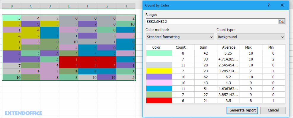
Μετρήστε γρήγορα / αθροίστε κελιά ανά χρώμα φόντου ή μορφής στο Excel

Σε ορισμένες περιπτώσεις, μπορεί να έχετε μια σειρά κελιών με πολλά χρώματα και αυτό που θέλετε είναι να μετρήσετε / αθροίσετε τιμές με βάση το ίδιο χρώμα, πώς μπορείτε να υπολογίσετε γρήγορα;
Με Kutools για Excel's Μετρήστε ανά χρώμα, μπορείτε να κάνετε γρήγορα πολλούς υπολογισμούς ανά χρώμα και επίσης να δημιουργήσετε μια αναφορά για το υπολογισμένο αποτέλεσμα.  Κάντε κλικ για δωρεάν πλήρη δοκιμαστική έκδοση σε 30 ημέρες!
αριθμός εγγράφων ανά χρώμα 1
 
Kutools για Excel: με περισσότερα από 300 εύχρηστα πρόσθετα Excel, δωρεάν δοκιμή χωρίς περιορισμό σε 30 ημέρες.

Τα καλύτερα εργαλεία παραγωγικότητας γραφείου

🤖 Kutools AI Aide: Επανάσταση στην ανάλυση δεδομένων με βάση: Ευφυής Εκτέλεση   |  Δημιουργία κώδικα  |  Δημιουργία προσαρμοσμένων τύπων  |  Αναλύστε δεδομένα και δημιουργήστε γραφήματα  |  Επίκληση Λειτουργιών Kutools...
Δημοφιλή χαρακτηριστικά: Εύρεση, επισήμανση ή αναγνώριση διπλότυπων   |  Διαγραφή κενών γραμμών   |  Συνδυάστε στήλες ή κελιά χωρίς απώλεια δεδομένων   |   Γύρος χωρίς φόρμουλα ...
Σούπερ Αναζήτηση: VLookup πολλαπλών κριτηρίων    VLookup πολλαπλών τιμών  |   VLookup σε πολλά φύλλα   |   Ασαφής αναζήτηση ....
Σύνθετη αναπτυσσόμενη λίστα: Γρήγορη δημιουργία αναπτυσσόμενης λίστας   |  Εξαρτημένη αναπτυσσόμενη λίστα   |  Πολλαπλή αναπτυσσόμενη λίστα ....
Διαχειριστής στήλης: Προσθέστε έναν συγκεκριμένο αριθμό στηλών  |  Μετακίνηση στηλών  |  Εναλλαγή κατάστασης ορατότητας κρυφών στηλών  |  Συγκρίνετε εύρη και στήλες ...
Επιλεγμένα Χαρακτηριστικά: Εστίαση πλέγματος   |  Προβολή σχεδίου   |   Μεγάλη Formula Bar    Διαχείριση βιβλίου εργασίας & φύλλου   |  Βιβλιοθήκη πόρων (Αυτόματο κείμενο)   |  Επιλογή ημερομηνίας   |  Συνδυάστε φύλλα εργασίας   |  Κρυπτογράφηση/Αποκρυπτογράφηση κελιών    Αποστολή email ανά λίστα   |  Σούπερ φίλτρο   |   Ειδικό φίλτρο (φίλτρο με έντονη γραφή/πλάγια γραφή/διαγραφή...) ...
Κορυφαία 15 σύνολα εργαλείων12 Κείμενο Εργαλεία (Προσθήκη κειμένου, Κατάργηση χαρακτήρων, ...)   |   50 + Διάγραμμα Τύποι (Gantt διάγραμμα, ...)   |   40+ Πρακτικό ΜΑΘΗΜΑΤΙΚΟΙ τυποι (Υπολογίστε την ηλικία με βάση τα γενέθλια, ...)   |   19 Εισαγωγή Εργαλεία (Εισαγωγή κωδικού QR, Εισαγωγή εικόνας από το μονοπάτι, ...)   |   12 Μετατροπή Εργαλεία (Αριθμοί σε λέξεις, Μετατροπή Συναλλάγματος, ...)   |   7 Συγχώνευση & διαχωρισμός Εργαλεία (Σύνθετες σειρές συνδυασμού, Διαίρεση κελιών, ...)   |   ... κι αλλα

Αυξήστε τις δεξιότητές σας στο Excel με τα Kutools για Excel και απολαύστε την αποτελεσματικότητα όπως ποτέ πριν. Το Kutools για Excel προσφέρει πάνω από 300 προηγμένες δυνατότητες για την ενίσχυση της παραγωγικότητας και την εξοικονόμηση χρόνου.  Κάντε κλικ εδώ για να αποκτήσετε τη δυνατότητα που χρειάζεστε περισσότερο...

Περιγραφή


Το Office Tab φέρνει τη διεπαφή με καρτέλες στο Office και κάνει την εργασία σας πολύ πιο εύκολη

  • Ενεργοποίηση επεξεργασίας και ανάγνωσης καρτελών σε Word, Excel, PowerPoint, Publisher, Access, Visio και Project.
  • Ανοίξτε και δημιουργήστε πολλά έγγραφα σε νέες καρτέλες του ίδιου παραθύρου και όχι σε νέα παράθυρα.
  • Αυξάνει την παραγωγικότητά σας κατά 50% και μειώνει εκατοντάδες κλικ του ποντικιού για εσάς κάθε μέρα!
Comments (21)
No ratings yet. Be the first to rate!
This comment was minimized by the moderator on the site
But If I want to sum a column range(say l7:l7800) out of the range d7:ct9000 based on the condition in column a(a7:a9000) and column b(b7:b9000). How will I do it. Please advise
This comment was minimized by the moderator on the site
Is there a way to create a dynamic ranged view, that will isolate all orders from a specific client within a list of clients? I have looked at multiple videos and none actually do what I need it to do. Is there a way to do this or would I need to pull the needed info into a controlled table and use the information from that table?
This comment was minimized by the moderator on the site
Hi, CareTaker. I do not get your question clearly. Could you describe your question or upload a file to show the quetion in details? But I recomend a utility called Data Association for you, maybe can help you, go to this web for details: https://www.extendoffice.com/product/kutools-for-excel/excel-click-cell-to-filter-based-on-another-workbook.html.
This comment was minimized by the moderator on the site
Thank you for the response, its quite the complicated thing to explain but I did manage to come right in the end using the indexing formula with the match formula as well.   =INDEX($B:$B;MATCH($C$2;$B:$B;0);):INDEX($N:$N;MATCH($C$2;$B:$B;0)+$C$3-1;)   at first it was confusing but I'm good now 
This comment was minimized by the moderator on the site
how do I update sum range by using helper cell...For example: if initial sum range is = C1 to M1, how to do change sum range if new data is up to AB1 using a helper cell, instead of changing the formula manually?
This comment was minimized by the moderator on the site
What if the rage is not column, but a row?
This comment was minimized by the moderator on the site
That's a bit trickier as I just found out. You need to use a combination of the CHAR function to convert a number to a letter, CONCAT to piece together a letter and number comprising a cell address, and the INDIRECT function to recognize strings as cell addresses.

In my example, I wrote the following expression:

=SUM(INDIRECT(CONCAT("F",ROW())):INDIRECT(CONCAT(CHAR(64+5+$B$31),ROW())))


where:
Row() is the current row
$B$31 is the cell where the # of columns to count is stored
5 is the offset for the first column to be counted

if you need to go beyond column Z, you’d need a less intuitive variant on that expression using the ADDRESS function:

=SUM(indirect(concat("F",row())):indirect(ADDRESS(row(),$B$31+5,4)))


where:
4 indicates a relative reference
This comment was minimized by the moderator on the site
Hi quick question. My formula =SUMIFS(DATA!$D$5:$D$13914,DATA!$E$5:INDIRECT(CONCATENATE("$E$",C3)),"<"&"1/1/2016") has a range that is from another tab called "DATA." I keep getting #VALUE! errors for this formula. Any suggestions? thanks!
This comment was minimized by the moderator on the site
Earlier I posted: Great formula but why does it only work when referring to the first cell. In other words, if you move the whole range down and the first cell in the range is A5 instead of A1, the formula ceases to work.
After playing with it, I figured out why the formula is not working when the starting row is not row 1. Excel interprets this as the range being A1 thru A4. If you are starting with a different row than row 1, here is how to modify the formula assuming the range now starts with A5:=MAX(A5:INDIRECT(CONCATENATE("A",ROW(A5)+B2)))
This works because the concatenation sees the row reference as fixed in the first example, but it becomes relative in the second example. Hope that helps!
Jared - You can just subtract 4 instead of adding. =MAX(A5:INDIRECT(CONCATENATE("A",ROW(A5)-B2))) [Assuming you have 4 in cell B2, or you could just leave the formula as is and put -4 in cell B2.]
This comment was minimized by the moderator on the site
Hi,cathy, thanks for your supplement, I have test your formula, I think the correct formula may be =MAX(A5:INDIRECT(CONCATENATE("A",ROW(A5)+B2-1))). I have update the tutorual. Thanks again.
This comment was minimized by the moderator on the site
Great formula but why does it only work when referring to the first cell. In other words, if you move the whole range down and the first cell in the range is A6 instead of A1, the formula ceases to work. That seems strange.
This comment was minimized by the moderator on the site
What if I want to count upward from a cell rather than downward? In the above example, the formula starts with A1 and goes downward. Let's say I want a range of 4 cells, beginning with Cell A10 and going to A6. Thank you!
This comment was minimized by the moderator on the site
Jared - See my most recent post for how to solve this.
This comment was minimized by the moderator on the site
I'm having this upward problem also but unable to see your other post for the solution. Can you give me link of the post please? Many thanks!
This comment was minimized by the moderator on the site
Hi, here is a formula may help you to calcualte upward.
=AVERAGE(INDIRECT(CONCATENATE("A",COUNT(A:A)-B1+1)):INDIRECT(CONCATENATE("A",COUNT(A:A))))
A:A is the column that you want to calcualte the average values, B1 is the cell that define the range in column A to calculate.
This comment was minimized by the moderator on the site
Thanks, but may I know why need to use "-B1+1" please?
This comment was minimized by the moderator on the site
Hi, Let me take a detailed example to explain it for you. There are 10 rows in column A, I want to get the last 2 values' average, in other words, average the values in row 9 and row 10. Now B1 contains 2, =COUNT(A:A)-B1+1 will get the result 9, COUNT(A:A) will get the result 10 (the last row of the column A). Now combine other functions to averaget the values in row 9 and row 10. Hope this can help you.
This comment was minimized by the moderator on the site
Can I use this syntax while referring to a different sheet?
This comment was minimized by the moderator on the site
If you want to sum referring to a Different Shet In CONCATENATE formula write [ SHEET NAME+COLUMN+ROW]
Formula=SUM(INDIRECT(CONCATENATE("Sheet1!","D",1)):INDIRECT(CONCATENATE("Sheet1!","D",5)))
This comment was minimized by the moderator on the site
Hi, Thank you so much for your help, but I have a small problem that is I don't have just one column but several ones (about 100 columns) is there a way to change the formula to accommodate the change in columns so O can get the sum for Columns A B C and so on. thanks for your help
This comment was minimized by the moderator on the site
Thank u for your message. If you want to sum first n values across multiple continuous columns, just change A to the last column you ues. EG, sum first 5 values across column A to column D, apply this formula =SUM(A1:INDIRECT(CONCATENATE("D",F2))).
There are no comments posted here yet
Please leave your comments in English
Posting as Guest
×
Rate this post:
0   Characters
Suggested Locations