Μετάβαση στο κύριο περιεχόμενο

Πώς να αθροίσετε με βάση τα κριτήρια στήλης και σειράς στο Excel; 

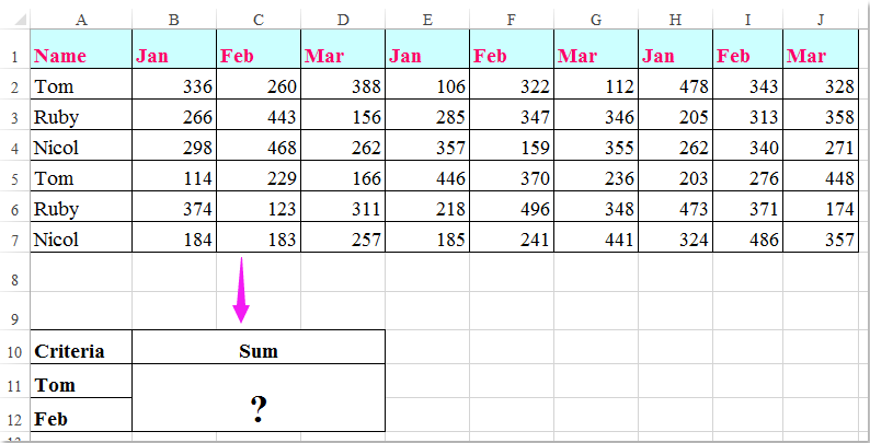
Έχω ένα εύρος δεδομένων που περιέχει κεφαλίδες γραμμής και στήλης, τώρα, θέλω να λάβω ένα άθροισμα των κελιών που πληρούν τα κριτήρια κεφαλίδας στήλης και γραμμής. Για παράδειγμα, για να συνοψίσουμε τα κελιά που τα κριτήρια στήλης είναι Tom και τα κριτήρια σειράς είναι Φεβρουάριος όπως φαίνεται στο παρακάτω στιγμιότυπο οθόνης. Αυτό το άρθρο, θα μιλήσω για μερικούς χρήσιμους τύπους για την επίλυσή του.

Κριτήρια σειράς στήλης doc άθροισμα 1

Αθροίστε τα κελιά με βάση κριτήρια στήλης και σειράς με τύπους


βέλος μπλε δεξιά φούσκα Αθροίστε τα κελιά με βάση κριτήρια στήλης και σειράς με τύπους

Εδώ, μπορείτε να εφαρμόσετε τους ακόλουθους τύπους για να αθροίσετε τα κελιά βάσει τόσο των κριτηρίων στήλης όσο και σειράς, κάντε το ως εξής:

Εισαγάγετε οποιονδήποτε από τους παρακάτω τύπους σε ένα κενό κελί όπου θέλετε να εξάγετε το αποτέλεσμα:

=SUMPRODUCT((A2:A7="Tom")*(B1:J1="Feb")*(B2:J7))

=SUM(IF(B1:J1="Feb",IF(A2:A7="Tom",B2:J7)))

Και στη συνέχεια πατήστε Shift + Ctrl + Enter πλήκτρα μαζί για να λάβετε το αποτέλεσμα, δείτε το στιγμιότυπο οθόνης:

Κριτήρια σειράς στήλης doc άθροισμα 2

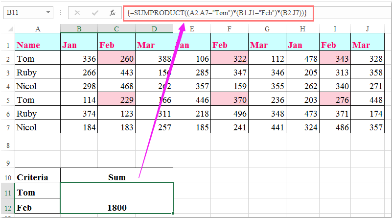
Note: Στους παραπάνω τύπους: τόμος και Φεβρουάριος είναι τα κριτήρια στήλης και σειράς που βασίζονται σε, A2: A7, Β1: J1 οι κεφαλίδες στηλών και οι κεφαλίδες σειράς περιέχουν τα κριτήρια, Β2: J7 είναι το εύρος δεδομένων που θέλετε να συνοψίσετε.

Τα καλύτερα εργαλεία παραγωγικότητας γραφείου

🤖 Kutools AI Aide: Επανάσταση στην ανάλυση δεδομένων με βάση: Ευφυής Εκτέλεση   |  Δημιουργία κώδικα  |  Δημιουργία προσαρμοσμένων τύπων  |  Αναλύστε δεδομένα και δημιουργήστε γραφήματα  |  Επίκληση Λειτουργιών Kutools...
Δημοφιλή χαρακτηριστικά: Εύρεση, επισήμανση ή αναγνώριση διπλότυπων   |  Διαγραφή κενών γραμμών   |  Συνδυάστε στήλες ή κελιά χωρίς απώλεια δεδομένων   |   Γύρος χωρίς φόρμουλα ...
Σούπερ Αναζήτηση: VLookup πολλαπλών κριτηρίων    VLookup πολλαπλών τιμών  |   VLookup σε πολλά φύλλα   |   Ασαφής αναζήτηση ....
Σύνθετη αναπτυσσόμενη λίστα: Γρήγορη δημιουργία αναπτυσσόμενης λίστας   |  Εξαρτημένη αναπτυσσόμενη λίστα   |  Πολλαπλή αναπτυσσόμενη λίστα ....
Διαχειριστής στήλης: Προσθέστε έναν συγκεκριμένο αριθμό στηλών  |  Μετακίνηση στηλών  |  Εναλλαγή κατάστασης ορατότητας κρυφών στηλών  |  Συγκρίνετε εύρη και στήλες ...
Επιλεγμένα Χαρακτηριστικά: Εστίαση πλέγματος   |  Προβολή σχεδίου   |   Μεγάλη Formula Bar    Διαχείριση βιβλίου εργασίας & φύλλου   |  Βιβλιοθήκη πόρων (Αυτόματο κείμενο)   |  Επιλογή ημερομηνίας   |  Συνδυάστε φύλλα εργασίας   |  Κρυπτογράφηση/Αποκρυπτογράφηση κελιών    Αποστολή email ανά λίστα   |  Σούπερ φίλτρο   |   Ειδικό φίλτρο (φίλτρο με έντονη γραφή/πλάγια γραφή/διαγραφή...) ...
Κορυφαία 15 σύνολα εργαλείων12 Κείμενο Εργαλεία (Προσθήκη κειμένου, Κατάργηση χαρακτήρων, ...)   |   50 + Διάγραμμα Τύποι (Gantt διάγραμμα, ...)   |   40+ Πρακτικό ΜΑΘΗΜΑΤΙΚΟΙ τυποι (Υπολογίστε την ηλικία με βάση τα γενέθλια, ...)   |   19 Εισαγωγή Εργαλεία (Εισαγωγή κωδικού QR, Εισαγωγή εικόνας από το μονοπάτι, ...)   |   12 Μετατροπή Εργαλεία (Αριθμοί σε λέξεις, Μετατροπή Συναλλάγματος, ...)   |   7 Συγχώνευση & διαχωρισμός Εργαλεία (Σύνθετες σειρές συνδυασμού, Διαίρεση κελιών, ...)   |   ... κι αλλα

Αυξήστε τις δεξιότητές σας στο Excel με τα Kutools για Excel και απολαύστε την αποτελεσματικότητα όπως ποτέ πριν. Το Kutools για Excel προσφέρει πάνω από 300 προηγμένες δυνατότητες για την ενίσχυση της παραγωγικότητας και την εξοικονόμηση χρόνου.  Κάντε κλικ εδώ για να αποκτήσετε τη δυνατότητα που χρειάζεστε περισσότερο...

Περιγραφή


Το Office Tab φέρνει τη διεπαφή με καρτέλες στο Office και κάνει την εργασία σας πολύ πιο εύκολη

  • Ενεργοποίηση επεξεργασίας και ανάγνωσης καρτελών σε Word, Excel, PowerPoint, Publisher, Access, Visio και Project.
  • Ανοίξτε και δημιουργήστε πολλά έγγραφα σε νέες καρτέλες του ίδιου παραθύρου και όχι σε νέα παράθυρα.
  • Αυξάνει την παραγωγικότητά σας κατά 50% και μειώνει εκατοντάδες κλικ του ποντικιού για εσάς κάθε μέρα!
Comments (17)
No ratings yet. Be the first to rate!
This comment was minimized by the moderator on the site
Brilliant!

The function =SUM(IF(B1:J1="Feb",IF(A2:A7="Tom",B2:J7))) is a great X & Y summation tool.
I would not have thought this logic out on my own.
In fact i took me a minute to deconstruction the operations.

Thank you
This comment was minimized by the moderator on the site
My data that I am trying to retrieve is in a table. Would this impact the result at all? I have:

=SUM(IF('[Primary Controller Active Project Database (KC notes)1.xlsx]Active Project Tracking'!$B2:$B66=X2,IF('[Primary Controller Active Project Database (KC notes)1.xlsx]Active Project Tracking'!$A1:$AV1=AH10,'[Primary Controller Active Project Database (KC notes)1.xlsx]Active Project Tracking'!$H$2:$AV$66)))

So I think the equivalent would be if you did your information above, but in a table in a different workbook. Thoughts?
This comment was minimized by the moderator on the site
If there were negatives in the matrix and you only wanted to include the positives, what would you do? 
I tried to do something like this:

=SUMPRODUCT((Column = Criteria)* ( Row = Criteria) * (second column = Criteria) * (Matrix) * (Matrix >0))

This comment was minimized by the moderator on the site
Is there a way to do this but instead of writing "Tom" & "Feb" in the formula, you are able to reference the criteria cells e.g.A11 & A12?
This comment was minimized by the moderator on the site
Hello, Rianna,Yest, as you said, you can use the cell references to replace the text in the formula, such as:
=SUMPRODUCT((A2:A7=A2)*(B1:J1=C1)*(B2:J7))
=SUM(IF(B1:J1=C1,IF(A2:A7=A2,B2:J7)))
This comment was minimized by the moderator on the site
In the above example which formula should I use if I wanted calculate the sum of the amounts earned by Tom Ruby & Nicol in March?
This comment was minimized by the moderator on the site
Hello, Nabar,To get the result you want, please apply the below formula:=SUMPRODUCT(((A2:A7="Tom")+(A2:A7="Nicol")+(A2:A7="Ruby"))*(B1:J1="Mar")*(B2:J7))
Please try, hope it can help you!
This comment was minimized by the moderator on the site
Hello Skyyang,
Thank you for your response. I tried the formula you suggested but I am not getting the right answer. Probably I wasn't able to put my query correctly. Let me try again I have a spreadsheet with data with daily calculation, I have numbered the first row 1,2,3,4.....132. 2nd, 3rd 4th &5th rows has table headings. The first column has line no's numbered 1, 2,3,.....3005 starting from row 6,range B6:EF3005 has data filled in on everyday basis. In second sheet i have a table in which I want to apply a formula which will look up two line numbers fed in two different rows and calculate the sum from the range B6: EF3005 from the data spreadsheet between the two line numbers from a certain column viz sum of values in column 15 between rows (line No's) 50 & 85.
This comment was minimized by the moderator on the site
Is there a way to make this work with wildcard characters? I'd like to use it on everything starting with certain characters, but with (a fixed number of) undefined characters at the end, i.e. =SUM(IF(B1:J1="Fe*",IF(A2:A7="To*",B2:J7)))
This comment was minimized by the moderator on the site
Should anyone have the same question, this is how I solved it (in Google Sheets, not tested in Excel):

=ArrayFormula(SUM(IF(regexmatch(O5:W5,"^Fe."),IF(regexmatch(N6:N11,"^To."),O6:W11))))

Note that the IF function does not support wildcard characters and that for regexmatch the wildcards are different and can be found here: https://github.com/google/re2/blob/master/doc/syntax.txt
In this particular instance, I used ^ to indicate that Fe & Tom occur at the beginning of text and . to allow for any following character (* would mean zero or more of the previous character, e.g. Fe* would only look for instances with 1 or more "e"s after F)
This comment was minimized by the moderator on the site
I tried to create a formula to calculate if the D12 is blank, it will calculate from K12 to AH12 but it seems this part ' regexmatch(D12,"")' is not working
ArrayFormula(SUM(IF(regexmatch(D12,""),K12:AH12)))
This comment was minimized by the moderator on the site
Thank you so much! You made my day!! @TeSageDS
This comment was minimized by the moderator on the site
how would you do this same formula if you wanted to sum both Feb and March together? please help! thanks

=SUMPRODUCT((A2:A7="Tom")*(B1:J1="Feb")*(B2:J7))
This comment was minimized by the moderator on the site
Hello,Angela,
To solve your problem, you just need to apply the below formula, please try it.

=SUMPRODUCT((A2:A7="Tom")*((B1:J1="Feb")+(B1:J1="Mar"))*(B2:J7)).

Hope it can help you!
This comment was minimized by the moderator on the site
Brilliant
This comment was minimized by the moderator on the site
Worth pointing out that of the two formulas provided above you do not need to enter the SUMPRODUCT formula with Ctrl + Shift + Enter. It will work perfectly well without it.
This comment was minimized by the moderator on the site
Awesome, this is the one what i was looking for. thanks for the help
There are no comments posted here yet
Please leave your comments in English
Posting as Guest
×
Rate this post:
0   Characters
Suggested Locations