Μετάβαση στο κύριο περιεχόμενο

Πώς να βρείτε το ένατο κενό κελί στο Excel;

Πώς θα μπορούσατε να βρείτε και να επιστρέψετε την nth μη κενή τιμή κελιού από μια στήλη ή μια σειρά στο Excel; Σε αυτό το άρθρο, θα μιλήσω για μερικούς χρήσιμους τύπους για να επιλύσετε αυτό το έργο.

Βρείτε και επιστρέψτε την nth μη κενή τιμή κελιού από μια στήλη με τύπο

Βρείτε και επιστρέψτε την nth μη κενή τιμή κελιού από μια σειρά με τύπο


βέλος μπλε δεξιά φούσκα Βρείτε και επιστρέψτε την nth μη κενή τιμή κελιού από μια στήλη με τύπο

Για παράδειγμα, έχω μια στήλη δεδομένων όπως φαίνεται το ακόλουθο στιγμιότυπο οθόνης, τώρα, θα λάβω την τρίτη μη κενή τιμή κελιού από αυτήν τη λίστα.

doc βρείτε nth μη κενό 1

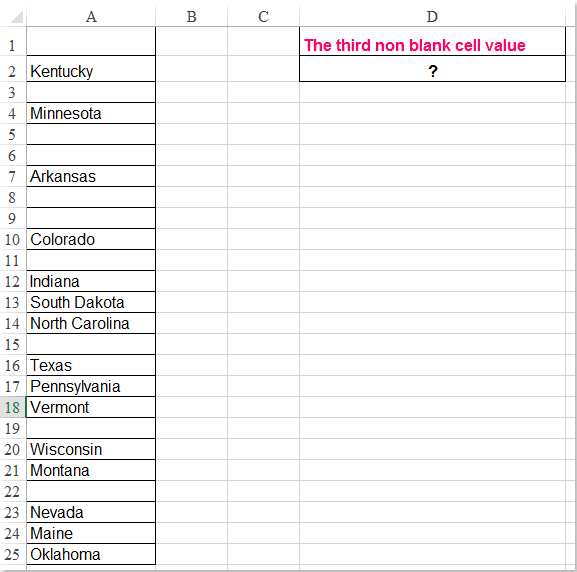
Εισαγάγετε αυτόν τον τύπο: =INDEX($A$1:$A$25,SMALL(ROW($A$1:$A$25)+(100*($A$1:$A$25="")), 3))&"" σε ένα κενό κελί όπου θέλετε να εξάγετε το αποτέλεσμα, D2, για παράδειγμα, και στη συνέχεια πατήστε Ctrl + Shift + Εισαγωγή πλήκτρα μαζί για να λάβετε το σωστό αποτέλεσμα, δείτε το στιγμιότυπο οθόνης:

doc βρείτε nth μη κενό 2

Note: Στον παραπάνω τύπο, A1: A25 είναι η λίστα δεδομένων που θέλετε να χρησιμοποιήσετε και ο αριθμός 3 υποδηλώνει την τρίτη μη κενή τιμή κελιού που θέλετε να επιστρέψετε, εάν θέλετε να λάβετε το δεύτερο μη κενό κελί, απλά πρέπει να αλλάξετε τον αριθμό 3 έως 2 όπως χρειάζεστε.


βέλος μπλε δεξιά φούσκα Βρείτε και επιστρέψτε την nth μη κενή τιμή κελιού από μια σειρά με τύπο

Εάν θέλετε να βρείτε και να επιστρέψετε την nth μη κενή τιμή κελιού στη σειρά, ο παρακάτω τύπος μπορεί να σας βοηθήσει, κάντε το εξής:

Εισαγάγετε αυτόν τον τύπο: =INDEX($A$1:$M$1,SMALL(IF($A$1:$M$1<>"",COLUMN($A$1:$M$1)-COLUMN($A$1)+1),4)) σε ένα κενό κελί όπου θέλετε να εντοπίσετε το αποτέλεσμα και, στη συνέχεια, πατήστε Ctrl + Shift + Εισαγωγή πλήκτρα μαζί για να λάβετε το αποτέλεσμα, δείτε το στιγμιότυπο οθόνης:

doc βρείτε nth μη κενό 3

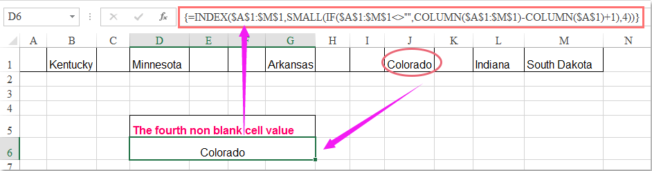
Σημείωση: Στον παραπάνω τύπο, Α1: Μ1 είναι οι τιμές γραμμής που θέλετε να χρησιμοποιήσετε και ο αριθμός 4 είναι η τέταρτη μη κενή τιμή κελιού που θέλετε να επιστρέψετε, εάν θέλετε να πάρετε το δεύτερο μη κενό κελί, απλά πρέπει να αλλάξετε τον αριθμό 4 έως 2 όπως χρειάζεστε.

Τα καλύτερα εργαλεία παραγωγικότητας γραφείου

🤖 Kutools AI Aide: Επανάσταση στην ανάλυση δεδομένων με βάση: Ευφυής Εκτέλεση   |  Δημιουργία κώδικα  |  Δημιουργία προσαρμοσμένων τύπων  |  Αναλύστε δεδομένα και δημιουργήστε γραφήματα  |  Επίκληση Λειτουργιών Kutools...
Δημοφιλή χαρακτηριστικά: Εύρεση, επισήμανση ή αναγνώριση διπλότυπων   |  Διαγραφή κενών γραμμών   |  Συνδυάστε στήλες ή κελιά χωρίς απώλεια δεδομένων   |   Γύρος χωρίς φόρμουλα ...
Σούπερ Αναζήτηση: VLookup πολλαπλών κριτηρίων    VLookup πολλαπλών τιμών  |   VLookup σε πολλά φύλλα   |   Ασαφής αναζήτηση ....
Σύνθετη αναπτυσσόμενη λίστα: Γρήγορη δημιουργία αναπτυσσόμενης λίστας   |  Εξαρτημένη αναπτυσσόμενη λίστα   |  Πολλαπλή αναπτυσσόμενη λίστα ....
Διαχειριστής στήλης: Προσθέστε έναν συγκεκριμένο αριθμό στηλών  |  Μετακίνηση στηλών  |  Εναλλαγή κατάστασης ορατότητας κρυφών στηλών  |  Συγκρίνετε εύρη και στήλες ...
Επιλεγμένα Χαρακτηριστικά: Εστίαση πλέγματος   |  Προβολή σχεδίου   |   Μεγάλη Formula Bar    Διαχείριση βιβλίου εργασίας & φύλλου   |  Βιβλιοθήκη πόρων (Αυτόματο κείμενο)   |  Επιλογή ημερομηνίας   |  Συνδυάστε φύλλα εργασίας   |  Κρυπτογράφηση/Αποκρυπτογράφηση κελιών    Αποστολή email ανά λίστα   |  Σούπερ φίλτρο   |   Ειδικό φίλτρο (φίλτρο με έντονη γραφή/πλάγια γραφή/διαγραφή...) ...
Κορυφαία 15 σύνολα εργαλείων12 Κείμενο Εργαλεία (Προσθήκη κειμένου, Κατάργηση χαρακτήρων, ...)   |   50 + Διάγραμμα Τύποι (Gantt διάγραμμα, ...)   |   40+ Πρακτικό ΜΑΘΗΜΑΤΙΚΟΙ τυποι (Υπολογίστε την ηλικία με βάση τα γενέθλια, ...)   |   19 Εισαγωγή Εργαλεία (Εισαγωγή κωδικού QR, Εισαγωγή εικόνας από το μονοπάτι, ...)   |   12 Μετατροπή Εργαλεία (Αριθμοί σε λέξεις, Μετατροπή Συναλλάγματος, ...)   |   7 Συγχώνευση & διαχωρισμός Εργαλεία (Σύνθετες σειρές συνδυασμού, Διαίρεση κελιών, ...)   |   ... κι αλλα

Αυξήστε τις δεξιότητές σας στο Excel με τα Kutools για Excel και απολαύστε την αποτελεσματικότητα όπως ποτέ πριν. Το Kutools για Excel προσφέρει πάνω από 300 προηγμένες δυνατότητες για την ενίσχυση της παραγωγικότητας και την εξοικονόμηση χρόνου.  Κάντε κλικ εδώ για να αποκτήσετε τη δυνατότητα που χρειάζεστε περισσότερο...

Περιγραφή


Το Office Tab φέρνει τη διεπαφή με καρτέλες στο Office και κάνει την εργασία σας πολύ πιο εύκολη

  • Ενεργοποίηση επεξεργασίας και ανάγνωσης καρτελών σε Word, Excel, PowerPoint, Publisher, Access, Visio και Project.
  • Ανοίξτε και δημιουργήστε πολλά έγγραφα σε νέες καρτέλες του ίδιου παραθύρου και όχι σε νέα παράθυρα.
  • Αυξάνει την παραγωγικότητά σας κατά 50% και μειώνει εκατοντάδες κλικ του ποντικιού για εσάς κάθε μέρα!
Comments (10)
No ratings yet. Be the first to rate!
This comment was minimized by the moderator on the site
CIAO STO CERCANDO DI APPLICARE LA TUA FORMULA MA NON MI FUNZIONA, DOVE STO SBAGLIANDO?
=INDICE($K$37:$K$88;MIN(RIGHE($K$37:$K$88)+RIGHE(100*($K$37:$K$88=""));6))&""
DEVO VISUALIZZARE L'ENNESIMA RIGA DIVERSA DA VUOTO

GRAzie
This comment was minimized by the moderator on the site
=INDICE($K$37:$K$88;MIN(RIGHE($K$37:$K$88)+(100*($K$37:$K$88=""));6))&""
This comment was minimized by the moderator on the site
I'm running this formula on a ~400 row sheet with around 20 blanks mixed throughout the data, and it's working perfectly EXCEPT when I fill the series down, it sometimes duplicates a row for some reason. For example, it seems to think a value is somehow simultaneously the 331st non-blank and the 332nd.

Things I've noticed:
-Duplications always happen in pairs (ex. 331 and 332 are duplicates, 333 and 334 will also be), then it goes back to normal for a while.
-Raw data also has blanks in pairs, but not corresponding to the duplicates
-No duplications occur in the first 94 rows, but they happen every 33-35 rows after that
-Does not appear to be linked to the value in the cell being duplicated
-I have entered as an array and as a standard formula, no difference in function

For reference, here's my actual formula:

=INDEX('PO Raw Data'!CR:CR,SMALL(ROW('PO Raw Data'!CR:CR)+(100*('PO Raw Data'!CR:CR="")),$W2)&"")

Note $W2 refers to a helper column and counts up as the data set is filled down, but only because I couldn't get it to count up when I just used a number instead of cell reference.
When I've replaced that cell reference (ex. $W2) with the appropriate number, same result.


Any thoughts on what I can do to fix that?
This comment was minimized by the moderator on the site
very helpful,
although when I return the nth non blank cell in a column set to DATE, the returned value appears as number(general number).formatting the cell into DATE also doesn't change the result. could you please give me a hand!
thanks a lot
This comment was minimized by the moderator on the site
Hello, Shirazi,
Sorry, maybe there is no direct formula for you to get the date format.

If someone else has the solution, please comment here.
This comment was minimized by the moderator on the site
Hi everyone!


Could you also help me return the row number of the second, third non-blank cell?


Please help me.
This comment was minimized by the moderator on the site
Hello, John,
the following formula can help you to get all the row numbers of the non-blank cells, please try it, thank you!
=IFERROR(ROW(INDEX($A$1:$A$12,SMALL(INDEX(NOT(ISBLANK($A$1:$A$12))*ROW($A$1:$A$12),0),COUNTBLANK($A$1:$A$12)+ROW(A1)))),"")
This comment was minimized by the moderator on the site
Hey everyone,

I have a table with numerous columns and rows. The rows have range names, and a description/location at the beginning of the row range with its own range, example "Building No.s". There are multiple Row Ranges/ Buildings. There are headers at the top of each columns for specific "Building Assembly Types". The table content is numeric quantities for each type "Building Assembly Type" for each specific "Building" description/location. There could be as many as (100) "Building Assembly Types" column headers but I will limit the assemblies to (10) per row range, so there will be numerous blank cells in each "Building No." range.

I have other summary tables set up for each "Building" that I want to pull the non-blank cells quantities to, along with the corresponding header "Assembly Type" for each "Building" with a (10) max "Assemblies" per page.

I can identify the non-blank cell quantities by use of the array formula above for rows. The problem I am having is identifying the header that corresponds to it.

Ultimately if I can identify the "Assembly" header, I can always index the "Quantities" once I have the header "Assembly" identified for each "Building". Then I would be able do a lookup for all the parts associated with each "Assembly" type for that "Building" from my Assembly parts database and multiply it times the "Quantity" of each assembly type.

Hopefully this makes since and someone can help.
This comment was minimized by the moderator on the site
Hello, I am looking for the third blank row in a column and I copied your formula and just changed the range from $A$1:$A:$25 to my range $D$306:$D$354. But when I change the range I get #REF! as my answer. I already converted to an array, control-shift-enter. Now the cell range I am referencing has formulas in them, so could that be why I am getting #REF. Your formula: =INDEX($A$1:$A$25,SMALL(ROW($A$1:$A$25)+(100*($A$1:$A$25="")), 3))&"" My formula: =INDEX($D$306:$D$354,SMALL(ROW($D$306:$D$354)+(1*($D$306:$D$354="")), 2))&"" Thanks, Noel
This comment was minimized by the moderator on the site
you have put the 1 instead of 100 therefore answered was wrong. please use below formula

INDEX($D$306:$D$354,SMALL(ROW($D$306:$D$354)+(100*($D$306:$D$354="")), 3))&"" than ctrl + shift+enter
There are no comments posted here yet
Please leave your comments in English
Posting as Guest
×
Rate this post:
0   Characters
Suggested Locations