Πώς να εμφανίσετε το αντίστοιχο όνομα της υψηλότερης βαθμολογίας στο Excel;

Υποθέτοντας ότι έχω εύρος δεδομένων που περιέχει δύο στήλες - στήλη ονόματος και αντίστοιχη στήλη βαθμολογίας, τώρα, θέλω να λάβω το όνομα του ατόμου που σημείωσε την υψηλότερη βαθμολογία. Υπάρχουν καλοί τρόποι αντιμετώπισης αυτού του προβλήματος γρήγορα στο Excel;

Εμφάνιση του αντίστοιχου ονόματος της υψηλότερης βαθμολογίας με τύπους

Εμφάνιση του αντίστοιχου ονόματος της υψηλότερης βαθμολογίας με τύπους

Για να ανακτήσετε το όνομα του ατόμου που σημείωσε την υψηλότερη βαθμολογία, οι παρακάτω τύποι μπορούν να σας βοηθήσουν να λάβετε το αποτέλεσμα.

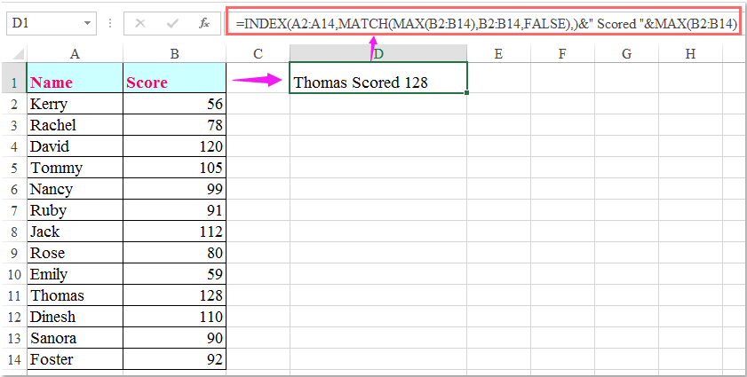
Εισαγάγετε αυτόν τον τύπο: =INDEX(A2:A14,MATCH(MAX(B2:B14),B2:B14,FALSE),)&" Scored "&MAX(B2:B14) σε ένα κενό κελί όπου θέλετε να εμφανίσετε το όνομα και, στη συνέχεια, πατήστε εισάγετε κλειδί για να επιστρέψετε το αποτέλεσμα ως εξής:

:

1. Στον παραπάνω τύπο, A2: A14 είναι η λίστα ονομάτων από την οποία θέλετε να λάβετε το όνομα και Β2: Β14 είναι η λίστα βαθμολογίας.

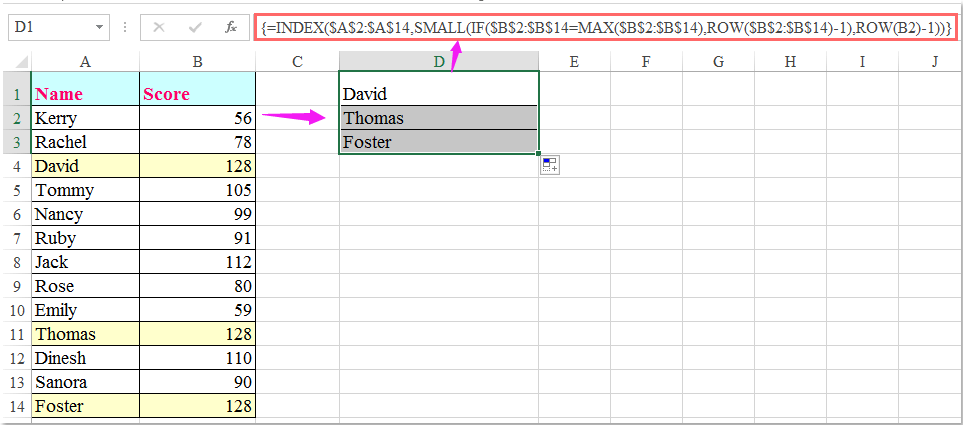
2. Ο παραπάνω τύπος μπορεί να πάρει το πρώτο όνομα μόνο εάν υπάρχουν περισσότερα από ένα ονόματα που έχουν τις ίδιες υψηλότερες βαθμολογίες, για να λάβετε όλα τα ονόματα που έχουν την υψηλότερη βαθμολογία, ο ακόλουθος τύπος πίνακα μπορεί να σας βοηθήσει.

Εισαγάγετε αυτόν τον τύπο:

=INDEX($A$2:$A$14,SMALL(IF($B$2:$B$14=MAX($B$2:$B$14),ROW($B$2:$B$14)-1),ROW(B2)-1)), και στη συνέχεια πατήστε Ctrl + Shift + Εισαγωγή πλήκτρα μαζί για να εμφανιστεί το όνομα, στη συνέχεια, επιλέξτε το κελί τύπου και σύρετε τη λαβή πλήρωσης προς τα κάτω μέχρι να εμφανιστεί η τιμή σφάλματος, εμφανίζονται όλα τα ονόματα που έλαβαν την υψηλότερη βαθμολογία όπως παρακάτω

Τα καλύτερα εργαλεία παραγωγικότητας γραφείου

🤖	Kutools AI Aide: Επανάσταση στην ανάλυση δεδομένων με βάση: Ευφυής Εκτέλεση   |  Δημιουργία κώδικα  |  Δημιουργία προσαρμοσμένων τύπων  |  Αναλύστε δεδομένα και δημιουργήστε γραφήματα  |  Επίκληση Λειτουργιών Kutools...
	Δημοφιλή χαρακτηριστικά: Εύρεση, επισήμανση ή αναγνώριση διπλότυπων   |  Διαγραφή κενών γραμμών   |  Συνδυάστε στήλες ή κελιά χωρίς απώλεια δεδομένων   |   Γύρος χωρίς φόρμουλα ...
	Σούπερ Αναζήτηση: VLookup πολλαπλών κριτηρίων  |   VLookup πολλαπλών τιμών  |   VLookup σε πολλά φύλλα   |   Ασαφής αναζήτηση ....
	Σύνθετη αναπτυσσόμενη λίστα: Γρήγορη δημιουργία αναπτυσσόμενης λίστας   |  Εξαρτημένη αναπτυσσόμενη λίστα   |  Πολλαπλή αναπτυσσόμενη λίστα ....
	Διαχειριστής στήλης: Προσθέστε έναν συγκεκριμένο αριθμό στηλών  |  Μετακίνηση στηλών  |  Εναλλαγή κατάστασης ορατότητας κρυφών στηλών  |  Συγκρίνετε εύρη και στήλες ...
	Επιλεγμένα Χαρακτηριστικά: Εστίαση πλέγματος   |  Προβολή σχεδίου   |   Μεγάλη Formula Bar   |  Διαχείριση βιβλίου εργασίας & φύλλου   |  Βιβλιοθήκη πόρων (Αυτόματο κείμενο)   |  Επιλογή ημερομηνίας   |  Συνδυάστε φύλλα εργασίας   |  Κρυπτογράφηση/Αποκρυπτογράφηση κελιών   |  Αποστολή email ανά λίστα   |  Σούπερ φίλτρο   |   Ειδικό φίλτρο (φίλτρο με έντονη γραφή/πλάγια γραφή/διαγραφή...) ...
	Κορυφαία 15 σύνολα εργαλείων:  12 Κείμενο Εργαλεία (Προσθήκη κειμένου, Κατάργηση χαρακτήρων, ...)   |   50 + Διάγραμμα Τύποι (Gantt διάγραμμα, ...)   |   40+ Πρακτικό ΜΑΘΗΜΑΤΙΚΟΙ τυποι (Υπολογίστε την ηλικία με βάση τα γενέθλια, ...)   |   19 Εισαγωγή Εργαλεία (Εισαγωγή κωδικού QR, Εισαγωγή εικόνας από το μονοπάτι, ...)   |   12 Μετατροπή Εργαλεία (Αριθμοί σε λέξεις, Μετατροπή Συναλλάγματος, ...)   |   7 Συγχώνευση & διαχωρισμός Εργαλεία (Σύνθετες σειρές συνδυασμού, Διαίρεση κελιών, ...)   |   ... κι αλλα

Αυξήστε τις δεξιότητές σας στο Excel με τα Kutools για Excel και απολαύστε την αποτελεσματικότητα όπως ποτέ πριν. Το Kutools για Excel προσφέρει πάνω από 300 προηγμένες δυνατότητες για την ενίσχυση της παραγωγικότητας και την εξοικονόμηση χρόνου.  Κάντε κλικ εδώ για να αποκτήσετε τη δυνατότητα που χρειάζεστε περισσότερο...

Διαβάστε περισσότερα ... ΔΩΡΕΑΝ Λήψη...

---

Το Office Tab φέρνει τη διεπαφή με καρτέλες στο Office και κάνει την εργασία σας πολύ πιο εύκολη

• Ενεργοποίηση επεξεργασίας και ανάγνωσης καρτελών σε Word, Excel, PowerPoint, Publisher, Access, Visio και Project.
• Ανοίξτε και δημιουργήστε πολλά έγγραφα σε νέες καρτέλες του ίδιου παραθύρου και όχι σε νέα παράθυρα.
• Αυξάνει την παραγωγικότητά σας κατά 50% και μειώνει εκατοντάδες κλικ του ποντικιού για εσάς κάθε μέρα!

Διαβάστε περισσότερα ... ΔΩΡΕΑΝ Λήψη...